Secular stagnation then and now
Secular stagnation refers to a prolonged and indefinite period of slow growth and high unemployment (or subnormal factor utilization). When was the last time this happened in the United States? Most people are likely to say the 1930s. In fact, it was the 1970s.
The 1970s were tumultuous years. There was the Vietnam war, oil supply shocks, and Watergate. The anchovies had disappeared off the coast of Peru. Clothing styles ranged from dreadful to appalling. Disco music was in. It was an awful time for those of us who lived through it.
The seventies are also known for a significant slowdown in measured productivity growth. (See Cullison 1989 for a useful review of issues related to measurement and interpretation). The most common measure of aggregate productivity is called Total Factor Productivity, or TFP for short (See Hulton 2000.)


The 1970s episode was called stagflation (an era of high inflation and high unemployment).
The two low-growth regimes above were different in an important way. When the economy transitions from a high to low-growth regime, the shock of regime change produces uncertainty. Investors will naturally move resources out of capital expenditure and into safer asset classes. Here is a critical question: What are the safe asset classes when a productivity slowdown occurs? The answer to this question seems to vary across episodes.
In the 1970s, the USD and UST securities were not among the set of safe assets. This was in large part due to the "unanchoring" of U.S. monetary policy following the breakdown of the Bretton Woods fixed exchange rate system. In August 1971, President Nixon announced that the USD would no longer be pegged to gold. More importantly than this, the public likely did not believe that monetary policy would keep inflation in check through other means (it took Volcker to convince the public of this several years later). The added fiscal pressures of the Vietnam war and the Great Society spending could not have helped this perception. As a result, the safe assets back then did not include government securities. Instead, investors flocked to assets outside the direct control of government, like gold and real estate.
In the most recent episode, real estate was most certainly not considered a safe asset. Investors began to walk away from real estate in 2006. They then ran way in 2008. Ironically, it was the USD and UST securities that proved to be among the most highly regarded assets this time around. This is no small part attributable to the fact that U.S. monetary and fiscal policies are presently perceived to be "anchored" (unsustainable paths for money and debt are viewed as temporary departures from a long-run stable anchor).
It's worth thinking about just how large the worldwide demand for U.S. money/debt must have grown since 2008. We can infer this enhanced demand from two observations. First, the supply of debt was increased substantially. Second, the price of that debt went up, not down (safe bond yields generally declined). What might have happened had the Fed/Treasury not intervened in the way they did?
To answer this latter question, we can look to the "hard money, tight fiscal" policy regimes in place when a low-growth regime hit the U.S. economy in 1929. In the early 1930s, short-term bond yields plummeted as today, and CPI inflation ran close to negative 10%. The unexpected and dramatic deflation--produced by an elevated demand for money against a fixed money supply--almost surely exacerbated the depth of the contraction through well-known channels.
The lesson here is that responsible monetary and fiscal policy "anchors" a regime, rendering its money/debt a safe asset. But anchoring a policy regime does not require strict adherence to a fixed asset supply rule, like the gold standard, or year-over-year balanced budgets. A credible regime will permit the supply of safe assets to expand "elastically" when the demand for the product is enhanced. Doing so can help stabilize inflation around its expected value. Of course, it is important to let the elastic snap back should economic conditions dictate. The experience of the 1970s demonstrates what can happen when a policy regime becomes unanchored.
The optimal conduct of monetary and fiscal policy over the longer term when a productivity slowdown hits is much less clear. Alvin Hansen expressed skepticism that expansionary monetary and fiscal policy could do much of anything beyond the initial shock period. If anything, it might even do some harm if, for example, such policies led to a very large public debt. Instead, Hansen favored what today we would label "pro-growth policies." His conclusions stemmed from the fact that he viewed growth slowdowns as the byproduct of slowing innovation and population growth--phenomena that monetary and fiscal policies are ill-equipped to deal with.
The situation is slightly different today in that, unlike in Hansen's time, there is presently a huge worldwide demand for U.S. treasuries. This demand stems from three major sources. First, the UST is used widely in the shadow banking sector (in repo and credit derivatives markets) as collateral, a sector that has grown significantly since the 1980s. Second, many emerging market economies want to hold USTs as a safe store of value. And third, there has recently been an added regulatory demand for USTs stemming from financial reforms like Dodd-Frank and Basel III. Because of these factors, it is likely that the U.S. economy can sustain a much higher debt-to-GDP ratio than it has in past.
Much of what one might recommend in terms of optimal policy stems from what is assumed to drive productivity (and population growth). For economies operating below the technological frontier (e.g., EMEs), productivity slowdowns might be avoided, in principle at least, through some type of policy change. However, the case is much less clear (to me) for economies operating near the technological frontier, where the Schumpetrian dynamic is more likely to govern the productivity dynamic. Some may point to the innovations produced during the second world war as example of how expansionary fiscal policy might enhance productivity growth. But surely, basic research and development can be better subsidized in a more targeted manner, without appealing to a massive and broad-based fiscal expenditure.
The 1970s were tumultuous years. There was the Vietnam war, oil supply shocks, and Watergate. The anchovies had disappeared off the coast of Peru. Clothing styles ranged from dreadful to appalling. Disco music was in. It was an awful time for those of us who lived through it.
The seventies are also known for a significant slowdown in measured productivity growth. (See Cullison 1989 for a useful review of issues related to measurement and interpretation). The most common measure of aggregate productivity is called Total Factor Productivity, or TFP for short (See Hulton 2000.)
Aside: What is TFP? Let Y denote the value of what is produced in an economy over the course of a year. Let (K,L) denote measures of the capital and labor services used to produce Y. Let F(K,L) denote an "aggregator function" that specifies the manner in which capital and labor are combined to form output. Given an assumed F and measurements on (Y,K,L), the TFP is computed as the residual TFP = Y/F(K,L). That is, the TFP measures the value of output unaccounted for by K and L. (Alternatively, think of TFP as measuring the average product of a list of factor inputs aggregated in a particular way.)The San Francisco Fed produces its own "utilization-adjusted TFP" series here. This is what what their measure of TFP looks like since 1960.
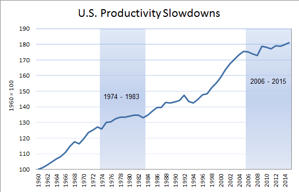
The shaded episodes were constructed using my eyeball metric, but I think that most people are likely to identify similar regions.
There is the matter of just how to interpret the productivity dynamic above. Personally, I find it hard to believe that productivity just grows in a straight line that the undulations we see above constitute measurement error. My own inclination is to interpret this pattern through a Schumpeterian lens (see here). Productivity growth appears in the form of growth-regimes. A productivity slowdown occurs when the economy switches from a high-growth regime to a low-growth regime. The economic shock is most pronounced in the first few years following a growth slowdown. (Related to this, see Zeira 1997.)
Economic theory suggests that the real rate of interest should (ceteris paribus) be low in a low-growth regime (and high in a high-growth regime). Let me compute a measure of the real rate of interest by taking the annual nominal yield on U.S. treasury debt and subtracting annual PCE inflation. Here is what the data looks like.

Well, not a perfect fit (remember the ceteris paribus part) but close enough, I think, to be intriguing. In particular, note that both low-growth regimes identified above are associated with significantly negative real interest rates. The early 1980s look odd by this view but, of course, we know that this era was associated with another type of regime change. In particular, Fed policy moved from a high-inflation regime to a low-inflation regime, with this regime change occurring in 1980 under Fed chair Paul Volcker.
Here is how the unemployment rate correlates with the real interest rate and growth regime.

Low-growth regimes beget low real interest rates and high unemployment rates. This seems consistent with Alvin Hansen's secular stagnation hypothesis (see my earlier post here). The pattern is evident in the most recent episode, as it is in the 1970s. Except nobody called it secular stagnation back then.
The 1970s may not be viewed as an era of secular stagnation because nominal interest rates and inflation were rather elevated in that episode. Secular stagnation, with its Depression-era origin, is more naturally related with low nominal interest rates and low inflation. But as the following diagram shows, secular stagnation can occur in high-inflation regimes as well as low-inflation regimes.

The 1970s episode was called stagflation (an era of high inflation and high unemployment).
The two low-growth regimes above were different in an important way. When the economy transitions from a high to low-growth regime, the shock of regime change produces uncertainty. Investors will naturally move resources out of capital expenditure and into safer asset classes. Here is a critical question: What are the safe asset classes when a productivity slowdown occurs? The answer to this question seems to vary across episodes.
In the 1970s, the USD and UST securities were not among the set of safe assets. This was in large part due to the "unanchoring" of U.S. monetary policy following the breakdown of the Bretton Woods fixed exchange rate system. In August 1971, President Nixon announced that the USD would no longer be pegged to gold. More importantly than this, the public likely did not believe that monetary policy would keep inflation in check through other means (it took Volcker to convince the public of this several years later). The added fiscal pressures of the Vietnam war and the Great Society spending could not have helped this perception. As a result, the safe assets back then did not include government securities. Instead, investors flocked to assets outside the direct control of government, like gold and real estate.
In the most recent episode, real estate was most certainly not considered a safe asset. Investors began to walk away from real estate in 2006. They then ran way in 2008. Ironically, it was the USD and UST securities that proved to be among the most highly regarded assets this time around. This is no small part attributable to the fact that U.S. monetary and fiscal policies are presently perceived to be "anchored" (unsustainable paths for money and debt are viewed as temporary departures from a long-run stable anchor).
It's worth thinking about just how large the worldwide demand for U.S. money/debt must have grown since 2008. We can infer this enhanced demand from two observations. First, the supply of debt was increased substantially. Second, the price of that debt went up, not down (safe bond yields generally declined). What might have happened had the Fed/Treasury not intervened in the way they did?
To answer this latter question, we can look to the "hard money, tight fiscal" policy regimes in place when a low-growth regime hit the U.S. economy in 1929. In the early 1930s, short-term bond yields plummeted as today, and CPI inflation ran close to negative 10%. The unexpected and dramatic deflation--produced by an elevated demand for money against a fixed money supply--almost surely exacerbated the depth of the contraction through well-known channels.
The lesson here is that responsible monetary and fiscal policy "anchors" a regime, rendering its money/debt a safe asset. But anchoring a policy regime does not require strict adherence to a fixed asset supply rule, like the gold standard, or year-over-year balanced budgets. A credible regime will permit the supply of safe assets to expand "elastically" when the demand for the product is enhanced. Doing so can help stabilize inflation around its expected value. Of course, it is important to let the elastic snap back should economic conditions dictate. The experience of the 1970s demonstrates what can happen when a policy regime becomes unanchored.
The optimal conduct of monetary and fiscal policy over the longer term when a productivity slowdown hits is much less clear. Alvin Hansen expressed skepticism that expansionary monetary and fiscal policy could do much of anything beyond the initial shock period. If anything, it might even do some harm if, for example, such policies led to a very large public debt. Instead, Hansen favored what today we would label "pro-growth policies." His conclusions stemmed from the fact that he viewed growth slowdowns as the byproduct of slowing innovation and population growth--phenomena that monetary and fiscal policies are ill-equipped to deal with.
The situation is slightly different today in that, unlike in Hansen's time, there is presently a huge worldwide demand for U.S. treasuries. This demand stems from three major sources. First, the UST is used widely in the shadow banking sector (in repo and credit derivatives markets) as collateral, a sector that has grown significantly since the 1980s. Second, many emerging market economies want to hold USTs as a safe store of value. And third, there has recently been an added regulatory demand for USTs stemming from financial reforms like Dodd-Frank and Basel III. Because of these factors, it is likely that the U.S. economy can sustain a much higher debt-to-GDP ratio than it has in past.
Much of what one might recommend in terms of optimal policy stems from what is assumed to drive productivity (and population growth). For economies operating below the technological frontier (e.g., EMEs), productivity slowdowns might be avoided, in principle at least, through some type of policy change. However, the case is much less clear (to me) for economies operating near the technological frontier, where the Schumpetrian dynamic is more likely to govern the productivity dynamic. Some may point to the innovations produced during the second world war as example of how expansionary fiscal policy might enhance productivity growth. But surely, basic research and development can be better subsidized in a more targeted manner, without appealing to a massive and broad-based fiscal expenditure.


0 comments:
Post a Comment